
"Modeling Bacterial Resilience" by Khoula Jaber
- Oct 20, 2023
- 20 min read
Updated: Oct 26, 2023
Modeling Bacterial Resilience: Simulation of Environmental Antibiotic Exposure to Substantiate the Predictive Power of Mathematical Model
Khoula Jaber, Joshua Harrington, Ph.D. and K. Joy Karnas, Ph.D., Cedar Crest College

Abstract: Antibiotic resistance has been a growing public health crisis made evident by the emergence of antibiotic resistant strains in clinical cases and environmental isolates. Overuse of antibiotics and their persistence in the environment provides a constant selective pressure that encourages the growth of resistant strains. The degree to which extended exposure leads to sustained resistance against antibiotics is a question that can be explored via mathematical modeling. Many models have been developed to predict the emergence of resistance, specifically utilizing derivative models over time to represent the rate of emergence of resistant isolates. The purpose of this project was to test the predictive power of published mathematical models by Ibargüen-Mondragon et al., 2014:

by simulating environmental exposure of a type-strain to the antimicrobial, triclosan. Using a 96-well plate design, we selected random individuals in a larger population of growth and monitored their growth in the presence and absence of triclosan. After confirming the predictive capabilities of the model, we broadened the scope of the study to explore both gram-positive and gram-negative bacterial species and included additional antibiotics. The ultimate goal of this project is to attain realistic modeling procedures, utilizing power series functions to depict change in bacterial growth more accurately over time.
Introduction
Antibiotic resistance has been an ongoing global health crisis as emergence of resistant strains increase and persevere in response to antibiotic exposure. Urgency on this issue has increased as the effectiveness of antibiotics commonly utilized for hospital-based infections decreases (Frieri et al., 2017). The emergence of resistant strains is due to genome alterations that lead to intracellular changes in biochemical pathways or extracellular changes that impact how the cell interacts with its environment. The high diversity of such resistance mechanisms has made it challenging to fully understand how acquired resistance in bacterial species occurs, especially when short term exposure to an antibiotic or multiple antibiotics results in novel resistance. There is no current solution for the resulting global health crisis due to antibiotic-resistant bacteria.
Combatting antibiotic resistance requires the discovery of novel drugs. In assessing the cost-benefit analysis of funding the discovery of new antibiotics, the initial cost is upwards of $55 billion for early drug target research (Dodds, 2017). Unfortunately, this investment has not yielded new classes of antibiotics in the past 50 years (Mutalik and Arkin, 2022). Additional countermeasures include the expansion of research in bacteriophage to bridge gaps in understanding of phage mechanisms and further expand applications of phage therapy (Mutalik and Arkin, 2022). It is also crucial that scientists have committed to a clear understanding of the precise mechanisms that lead to antibiotic resistances, especially those that result from constant exposure that serve as a selective pressure for microbes.
Antimicrobials found in a wide variety of consumer products have been targeted as causative agents driving antibiotic resistance due to their constant presence in the environment. This is observed with the antimicrobial, triclosan, which was previously found in many cleaning, cosmetic, plastic, and textile products (FDA, 2019). Due to the non-biodegradable nature of triclosan, it has collected in wastewater and groundwater systems in the United States, and thus the Food and Drug Administration (FDA) deemed the antimicrobial as a non-qualifier for “generally recognized as safe and effective” designation (FDA, 2016). Following this new classification of the drug, it was banned from FDA-approved products in 2017, however, due to its constant usage starting from the 1970’s, accumulation in the environment has resulted in resistance in environmentally isolated microbes (Welsch and Gillock, 2014; Marotta, 2018). Research on molecular mechanisms that lead to triclosan resistance has been conducted for decades. The initial mutation of the triclosan target site was documented in 1999, as the FabI[G93V/S] mutation (Heath et al.,1999). Additional resistance mechanisms such as efflux pump overexpression, specifically that of the acrAB operon, and overexpression of the multiple antibiotic resistance gene regulator, marA, have been documented (McMurry et al., 1998). While it is important to understand the molecular mechanisms that allow for antimicrobial resistance, it is crucial also to better understand the timeline of resistance.
Mathematical modeling can be used to predict required exposure periods before microbes develop resistance to antimicrobials. Logistic growth equations have been utilized to model many biological systems, and continuations of these equations have served to model population reducing or enhancing factors such as predator-prey interactions, interspecific competition, and intraspecific competition (Tsoularis and Wallace, 2002). Further, models utilizing residual power series methods have shown high accuracy and efficiency in modeling non-linear population growth patterns (Dunnimit et al., 2020). In bacterial species, the Lotka-Volterra model has been utilized to model interactions amongst bacterial species where resistance emergence in a given species of interest could be determined (Stein et al., 2013). Proposed continuation models have emphasized essential components required to model resistance effectively, including antibiotic consumption, concentration of antibiotic, and bacterial species relationships (Arepyava et al., 2017; Stein et al., 2013). A mathematical model capturing a wide variety of such variables and factors was introduced by Ibargüen-Mondragon et al. (2014) where the following models were utilized to determine antibiotic resistance in Mycobacterium tuberculosis:

Utilizing this modeling pair, resistance to antibiotics was predicted and further documented as an accurate modeling procedure in determining emergence of resistant bacterial strains.
This study seeks to identify a mathematical model which displays population change over time in presence of an antibiotic as a selective pressure. The model displayed above was identified from paper by Ibargüen-Mondragon et al., 2014. We aim to dissect the model and identify variables and values that can be modeled in real time. Further, we want to derive the model and identify/calculate variables identified. We would also like to mimic experimental parameters outlined in literature by designing growth experiments for microbes of interest. In addition to deriving the model, we want to apply model and experimental parameters to fast growing microbes as compared to slow growing microbes utilized in literature and model population changes over time to determine trends between different species and antibiotics.
Derivation of Proposed Mathematical Model:
The models introduced by Ibargüen-Mondragon et al. (2014) are displayed below:

To understand how the models were assembled, we started deriving an exponential growth model:

Where N is the current population size at time t, N0 is the starting population, and r is the growth rate.
Taking the derivative and introducing the concept of carrying capacity, we end with the following logistic growth model:

For competing populations, a competition coefficient must be introduced as the effect of one population on another. So, for coexisting populations in the same environment, call them N1 and N2 with competition coefficients a12, which is the effect of population 1 on population 2, and a21, which is the effect of population 2 on population 1.
Incorporating this into the model, we have:

Note, for our experimental purposes, we are deriving one population from another. That is, we are designing our experiment such that we are starting with a single uniform population, and introducing a selective pressure that will cause the emergence of another population that can grow in the presence of the selective pressure. This emergence is recorded over a short period of time (~16 hours) where it is highly unlikely that one population will have any notable advantage over the other. Considering both the source of one of the populations and considering the short period of selective pressure introduction, we can assume the following:

Therefore, we are left with:

If we replace N1 with S, and N2 with R, we have:

We are left to consider death rate, (μ) and mutation rate, (q). These two variables can be introduced at the end of each model as follows:

Now comparing this to the initially proposed models, we are left with the exclusion of death by antibiotic (α) and multiplying the concentration by the mutation rate, (qCS).

Methods:
Three strains were utilized in this study. The strain descriptions and storage conditions are as follows: Enterobacter cloacae ATCC 13047 (denoted ENC). Stocks were maintained in Luria-Bertani liquid broth at 37° C to achieve saturated culture/maximum growth. Staphylococcus aureus Wards Science 0299 (denoted SA). Stocks were maintained in Luria-Bertani liquid broth at 37° C to achieve saturated culture/maximum growth.. Escherichia coli ATCC 25922 denoted (EC). Stocks maintained in Luria-Bertani liquid broth at 37° C to achieve saturated culture/maximum growth with700 μL culture placed in 300 μL 50% glycerol and stored at -80° C.
Determination of Model Variables and Values:
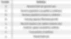
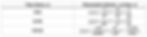
Variables introduced in the models are defined in the tables below, first what their symbol represents, (Table 1) and specific mathematical values fit in each variable’s place as determined by the researcher to best fit this study (Table 2).

Calculation of Antibiotic Uptake Rate (α) via Disk Diffusion:
Antibiotic uptake rate (death by antibiotic) calculations were done using disk diffusion assays with incrementally increasing concentrations of antibiotic on a 6 mm paper disk. This assay follows a traditional Kirby-Bauer (disk diffusion) set-up, with additional antibiotic disks utilized on the same plate to develop a linear relationship between concentration and death by antibiotic. Type strains of each species of interest (E. coli, En. cloacae, S. aureus) were grown in 5 mL Luria-Bertani (LB) broth to OD600 of 0.5 (mid-log). Using a cotton swab, each strain was separately plated on a Mueller-Hinton agar plate by soaking the swab with liquid culture and streaking the entire plate. Disks (6 mm) containing antibiotic(s) of interest (one antibiotic per plate) in varying concentrations (ug/mL) were placed on their designated plate. Disks were separated accordingly to allow proper and complete diffusion of each disk without interference of disks with each other. The plates were placed in 37° C incubator overnight (~16-24 hours). Afterwards, plates were removed, and zones of inhibition were measured. Zone of inhibition was the diameter across the circular zone where growth of the bacteria was inhibited. To graph the relationship between concentration and zone of inhibition, the log (base 10) of the concentration on the antibiotic disk was graphed against the zone of inhibition measurements (cm). A trendline was then designed to fit the data points output from each run. The slope of the line indicated the uptake rate as ug/cm. To properly convert this to cells taking up and dying from antibiotic exposure, cell size was considered. Both E. coli and En. cloacae cells fall in the range of 1.0-2.0 um in cell diameter, where S. aureus falls around 1.0 um in diameter (Riley, 2013). Therefore, the death by antibiotic calculation indicates the quantity of cells that did not survive due to antibiotic exposure (Table 3).

Calculation of Natural Death Rate (μ) via Exponential Decay:
The exponential decay formula found in the literature (Assadian et al., 2011) is recorded as:

Variables were altered to maintain uniform trend in variable identifications. Here “N” is a general population. Solving for μ,

Death rate was reported in cells/hr.
Sources: Determining values of β, K, and q
β, K and q were determined from literature values. The birth rate (β) was determined from the exponential growth rate of E. coli in Luria-Bertani broth. The growth rate of E. coli was recorded in time it takes to double the number of E. coli cells, which is 20 minutes (Gibson et al., 2018). Escherichia coli and En. cloacae are both from the Enterobacteriaceae family and their growth rates were recorded as relatively similar (Khleifat et al., 2008). The growth rate of Staphylococcus aureus was documented as a doubling time every 20 minutes (Missiakas and Schneewind, 2018).
Determining Antibiotic Concentrations:
The lowest concentration of an antimicrobial that will inhibit the visible growth of a microorganism after overnight incubation is the minimum inhibitory concentration (MIC) (Andrews JM, 2001). Triclosan solution was made in 8M NaOH and distilled water. NaOH was required to maintain the compound in solution in water. An additional note was that NaOH, in high amounts, made liquid LB broth very cloudy, rendering any absorbance readings as a means of growth essentially useless since the opacity of the NaOH + LB was much higher than that of a saturated culture. With this in mind, low concentrations of triclosan were utilized to ensure little to no effect on absorbance readings collected throughout the experimental process. The maximum concentration of triclosan utilized was 200 ug/mL, and the minimum concentration was 0.5 ug/mL. A starting stock solution of 20 mg/mL was maintained at 4° C. Antibiotic was diluted directly in LB broth to ensure no background NaOH was added to the solution. As a threshold for measure, the minimum inhibitory concentration (MIC) of triclosan was documented as 0.5 ug/mL in E. coli, and 0.125 ug/mL in S. aureus in ATCC derived strains (Assadian et al., 2011).
Chloramphenicol solid was diluted in 100% EtOH. To maintain consistency, the starting stock solution of chloramphenicol was at a concentration of 20 mg/mL. The maximum concentration of chloramphenicol used was 2 mg/mL, and the minimum concentration was 0.5 ug/mL. The MIC of chloramphenicol against E. coli was documented as 8 ug/mL (Pitsiniaga and Sullan, 2022). Chloramphenicol is light sensitive, so additional precautions were taken to ensure tubes were not left out in the light, and stock solutions (as well as diluted solutions) were stored at 4° C when not in use (Sigma Aldrich).
Erythromycin solid was diluted in 100% EtOH. To maintain consistency, the starting stock solution of erythromycin was at a concentration of 20 mg/mL. The maximum concentration of chloramphenicol used was 2 mg/mL, and the minimum concentration was 0.5 ug/mL. The MIC of erythromycin against S. aureus was documented as 0.25 ug/mL (Mikliasinska-Majdanik et al., 2022). Erythromycin is light sensitive, so additional precautions were taken to ensure tubes were not left out in the light, and stock solutions (as well as diluted solutions) were stored at 4° C when not in use (Sigma Aldrich).
Designing Growth Plate:
All samples in this experiment were initially grown at 37° C with constant shaking until the mid-log phase was achieved as determined by spectrophotometric measurement of the optical density of the culture via absorbance at 600 nm (OD600 of 0.5). The cultures were then combined 1:1 with LB or LB/antibiotic in a 96-well culture plate. These samples were incubated at 37° C with constant shaking to ensure uniform distribution of the cells and circulation of oxygen across the given time period (approximately 16 hours). During with OD600 measurements were recorded every five minutes.
Converting Optical Density to Cell Count:
To convert to cells/mL, a reference measurement of OD600=1 was utilized. At an OD of 1, the documented cell count was 8 x 10⁸ cells/mL (Agilent). The remaining calculations for readings between and OD of 0 and 1 were calculated using the conversion factor:

Determining Expected Growth Values: Excel Design:
The expected growth values were calculated in Excel by modeling change in population over time given the determined variables. Each determined variable was placed in a starting cell at the top of the Excel sheet, and equations for each variable were shown below where population development was modeled continuously as t, R, and S changed. Ending calculations were in terms of total population size, R+S.
The terms that were initially introduced in the Excel sheet were:
1. Starting population à OD600=0.5, which yielded 4.0 x 10⁷ cells/100 μL
2. Further, the starting population was diluted by 100 μL from the starting media in the plate, setting our starting population at 2.0 x 10⁷ cells in 200 μL.
3. The birth rate in the exponential growth equation, N=N0ert, “r” was calculated as ln(2)/tD, where “tD” is the desired time interval of growth, where this term would be 16 hours. Therefore, the bacterial growth rate would be r=0.02 after performing this calculation (Widdel, 2010). This was considered in each step of the population growth.
4. The mutation rate was set in a range, between 10-8 and 10-5 mutations per generation. The emergence of resistant individuals was set to either the upper or lower bound mutation rate(s) as separate experimental simulations. The genome length was incorporated into the mutation calculation, however, since the genomes differed by only a few hundred thousand base pairs, (E. coli 5,209,985 bp; En. cloacae 5,608,020 bp; S. aureus 2,729,352 bp), the approximation of genome length utilized was 5.5 million bases. The ending population (expected) did not change noticeably due to the low mutation rate being incorporated.
5. The carrying capacity was determined at 2.4 x 10⁹ cells/mL (Voklmer and Heinemann, 2011). In an experiment being run in 200 μL, our new carrying capacity would fall at 4.8 x 10⁸ cells.
6. The death rate, as explained previously, was incorporated as cells lost per hour and were subtracted off each population size before total population size was determined.
7. Knowing that bacterial growth hits stationary phase after 10 hours of growth, the Excel Design was marked to hit maximum growth at 10-11 hours of growth. This assumption is based on previous LB growth assays to help determine when growth would flatline.
Determining Ending Population Size (R+S): Growth Curve Analysis:
The final population size (R+S) in each experiment was determined by inputting known variables into Excel, and the total S and R individuals at each time point were calculated and then computed as a total population size. This calculation resulted in our expected growth. The actual growth values were determined via observing the pattern of change in each growth curve. Knowing we have limited resources in these experiments, the final population was determined when the growth curve flatlined after its observed exponential growth phase.
The final population was determined by subtracting the blank LB+ antibiotic well from the wells containing growth. Since each experiment was conducted in triplicate, the three were averaged after subtracting the blank from each experimental run. Then, the initial absorbance value was subtracted off each absorbance value at each time point. To convert the absorbance to cell count, we established in the “Converting Optical Density to Cell Count” the conversion factor of OD600=1=8 x 10⁸ cells/mL.
Analysis of Population Growth: Polynomial Representation:
Modeling population dynamics was done in three time frames for each experiment. To model population dynamics, three distinct regions of the growth curve were identified in each experiment and correlated to the three phases of bacterial growth: exponential growth phase, lag phase, and stationary phase. Observing the characteristics of the curve, exponential growth phase and lag phase can be modeled using different quadratic formulas. The transition of lag into stationary phase can be modeled using a cubic polynomial.
To do this, there were three to four points selected within each designated time frame. Using these points, a system of equations was set using fixed coefficients and constants. For example, selecting three points: P1, P2, P3 would have respective x and y values, where P1=(x1, y1); P1=(x2, y2); P3=(x3,y3). With these defined points, we can define fixed coefficients and constants a, b, c,…,z. So, for a quadratic representation, we had a system similar to the following:
ax12 +bx1 +c=y1
ax22 +bx2 +c=y2
ax32 +bx3 +c=y3
Similarly, for a cubic representation, we had:
ax13 +bx12 +cx1 +d=y1
ax23 +bx22 +cx2 +d=y2
ax33 +bx32 +cx3 +d=y3
Solving for a, b, c, and d can be done by separating the known variables into a matrix, and the unknowns (coefficients) into a coefficient matrix. For example, we would have the following matrix representation for a quadratic system:

For a cubic system, we had the following representation:

CoCalc®: Designing & Solving for Polynomial Coefficients:
CoCalc® utilizes Sage Math (which is an open library for coding with Python) to process codes entered by a user and generates a response, displayed below the entry box. In our case, we can solve our system of equations utilizing the “solve” function. The “solve” function in CoCalc® allows us to type in a system of equations after defining our variables, and simply typing in the variables CoCalc® should solve for. To define our variables, we simply input var (‘a, b, c’) to indicate these are variables we are solving for. The integers in the equation above would be our three points (P1, P2, P3) in each given time frame where each x value would be multiplied by the a, b, or c coefficients and the y value would be on the right side of the equation.
Three representations for each population were determined, at three different time frames as described above. When inputting the starting data values, the y values of each experiment were reduced by a factor of 108 to ensure coefficients were calculated within reasonable range.
Results
Growth Analysis: Expected Growth (Raw Values) vs. Actual Growth (Population Capacity):
The expected growth values were determined in Excel, as determined prior, the only difference between each of the microbes that could be calculated for was their genome length, and the final population growth determined at the end of the exponential growth phase entering into lag phase was between 2.36 x 10⁸ cells/mL and 2.86 x 10⁸ cells/mL. These raw growth values were compared against the expected growth values, averaging these values landed a final expected population growth value of 2.61 x 10⁸ cells/mL. This ending population size is the total of the sensitive strain and resistant strain growth. The actual population growth of each experiment was determined at the final population growth in each experiment. The final population size was determined at the final cells/mL value after 16 hours of growth. Table 4 shows all ending population sizes for each experiment.

Comparing expected and actual growth values, we see that expected growth fell around 2.61 x 10⁸ cells/mL. The general trend in each population representation shown above related closely to the expected growth values for each experiment, as shown, where En. cloacae was the closest in growth with chloramphenicol, and S. aureus with triclosan.
Polynomial Representations: Numerical Analysis:
In each of the experiments below, the polynomial representations are plotted against the experimental results shown in Table 4. Numerical analysis of each polynomial will be shown in the tables below within each time frame listed. In each time frame, the following times were used to generate all of the polynomials in the tables below. At time frame (0,4) hours 1, 2, and 3 were used. In frame (4,10) times 6, 8, and 10 were used. At frame (10,16) the times 12, 14, 16 were used. This follows for each polynomial generated. Three polynomials were developed against the growth curve for this experiment as shown in the table below, on the left is the time interval the polynomial represented, on the right is the polynomial representing the growth of this population (cells/mL) within that given time range.
Escherichia coli
In E. coli, polynomial representations were developed against the actual growth values collected in the presence of triclosan.

Enterobacter cloacae
In En. cloacae , polynomial representations were developed against the actual growth values collected in the presence of triclosan, chloramphenicol, and erythromycin. Note, erythromycin should not impact the growth of En. cloacae since it is a gram-positive specific antibiotic placed in the presence of a gram negative microbe.

Staphylococcus aureus
In S. aureus, polynomial representations were developed against the actual growth values collected in the presence of triclosan, chloramphenicol, and erythromycin. Note, chloramphenicol should only mildly impact the growth of S. aureus since it is mostly effective against gram-negative microbes and S. aureus is a gram-positive microbe.


Model Limitations
Variable Compatibility:
An initial note made was the lack of evidence supporting the multiplication of the mutation rate and antibiotic concentration. The variables were deemed incompatible, and it was further concluded that the product of the two variables does not necessarily follow the trend suggested by the model. That is, higher antibiotic concentrations would mean more sensitive individuals would mutate and become resistant. The three antibiotics researched in this project, as well as the antibiotics identified initially in literature are not mutagenic. That is, they do not induce DNA damage or mutations in the bacterial genome. However, although the evidence supporting the product of these variables is lacking, ignoring this aspect of the model was only a temporary approach until further clarification is developed.
Additionally, the death by antibiotic variable was introduced into the model in simplified form, a potential solution to this would be to expand the equation in order to effectively exclude the concentration times mutation rate calculation without excluding additional variables:

Including this death rate, along with the intrinsic death rate may help better model the emergence of resistant individuals while modeling the death of sensitive individuals.
Newly Proposed Model (Excluding Antibiotic Concentration):
Using the initial derivation, we performed to reach the model we investigated in literature, our initial proposed model for resistant and sensitive individuals were:

After determining a workaround to exclude the “qCS” variable while also including as many variables as was first introduced in the model as possible, we ended with:

Credibility & Limitations of New Model:
The limitations of this new model do not include all variables that were initially introduced by Ibargüen-Mondragon et al. (2014). Due to the concerns initially presented as having incompatible variables combined into a single term, there was no proper reasoning developed or found as to why the “qCS” term was incorporated in both the dR/dt and dS/dt model.
Modeling Population Dynamics
Accuracy of Polynomial Representations:
Each polynomial representation generated for each population was cross tested with each population of interest, yielding expected accuracy in the time frame it was meant to model. Initial plans to cross test representations across different species and different populations within similar species were developed and in progress of investigation. To cross test these polynomials, the outputs of each polynomial were cross-referenced with actual experimental growth.
Discussion
The initial derived model for dS/dt and dR/dt excluding the qCS term was relatively accurate in determining emergence of resistance by effectively maintaining similar ending R+S population sizes. While this model does not indicate how fast a bacterial strain can become resistant to an antibiotic, it can tell us how many resistant microbes can emerge within a given time range, effectively determining the ease of resistance given proper selective pressures and growth conditions. With high antibiotic concentrations, the derived model would not have accurately modeled emergence of resistant strains since there would be no growth observed due to the selective pressure being too high. Since none of the antibiotics investigated in this study were involved in mutagenic pathways, high concentrations of antimicrobials would serve to simply kill the entire bacterial population investigated. Therefore, the initially proposed model by Ibargüen-Mondragon would be more feasible if the studied antimicrobials were mutagenic. However, due to the nature of our selected antimicrobials, the model without the “qCS” term served to follow a more reasonable modeling method.
Exposing microbes to lower antibiotic concentrations was necessary in ensuring the emergence of resistant individuals would occur. In these experiments, the MIC of each antibiotic on each specific species was determined and used to create a range that was large enough to establish a range of proper experiments where resistant emergence was at high level enough to be noted (Wistrand-Yuen et al., 2018). Initially, Ibarguen-Mondragon, et al. (2014) had utilized this model in resistant strains of Mycobacterium tuberculosis, which is a slow growing microbe. The microbes investigated in this study were fast growing microbes and were effectively modeled regardless of their alternative growth nature. We were able to establish proper experimental procedures as well as predict resistance emergence over time effectively with derived logistic growth models, and thus are confident in the predictable nature of these growth models and can attest to its malleability in use against different populations.
Future work will develop more efficient methods in modeling population changes instead of using multiple polynomial representations. Although this technique is highly effective and accurate, it can be time consuming, especially if different populations tend to follow similar trends. We would also like to extend experimental parameters. The experiments in this project were designed in a 96-well plate that holds a maximum of 200 μL volume. To allow for more variation and potential uniqueness in each population’s trend, we would like to run experiments in much larger volumes such as 50 mL. This parameter extension may also serve to extend the time of experiments to last days instead of hours. Finally, we would like to increase the different types of microbes investigated to further increase the diversity of this experiment.
Acknowledgements
Thank you to the Department of Biological Sciences, Department of Mathematics, and the Honors Program for allowing me to conduct my research. A special thanks to Dr. Kliman for his support and guidance throughout the entirety of the experimental development and review process. Thank you to Dr. Jenny Hayden for her guidance and to Aisling Doyle for her help and for providing us with bacterial strains and antibiotics. Thank you to my colleagues, Sydney Jones, Audra Bratis, Megan Dunkle, and Patsy Holtz for their relentless support throughout this process.
References
Agilent. E. coli Cell Culture Concentration from OD600 calculator.
Andrews JM. 2001. Determination of minimum inhibitory concentrations. Journal of Antimicrobial Chemotherapy. 49(6): 1049
Arepyava MA, Kolbin AS, Sidorenko SV, Lawson R, Kurylev AA, Balykina YE, Mukhina NV, Spiridonova AA. 2017. A mathematical model for predicting the development of bacterial resistance based on the relationship between the level of antimicrobial resistance and the volume of antibiotic consumption. Journal of Global Antimicrobial Resistance. 8: 148-156
Assadian O, Wehse K, Hubner NO, Koburger T, Bagel S, Jethon F, Kramer A. 2011. Minimum inhibitory (MIC) and minimum microbiocidal concentration (MMC) of polyhexanide and triclosan against antibiotic sensitive and resistant Staphylococcus aureus and Escherichia coli strains. GMS Krankenhhyg Interdiszip. 6(1)
Dawkins P. 2023. Augmented Matrices. Math Lamar. Online Notes.
Dodds R. David. 2017. Antibiotic resistance: A current epilogue. Biochemical Pharmacology. 134: 139-146
Dunnimit Patcharee, Wiwatwanich A, Poltem D. 2020. Analytical Solution of Nonlinear Fractional Volterra Population Growth Model Using the Modified Residual Power Series Method. Symmetry. 12(11):1779.
Frieri Marianne, Kumar K, Boutin A. 2017. Antibiotic Resistance. Journal of Infection and Public Health. 10(4): 369-378
Gibson B, Wilson DJ, Feil W, Eyre-Walker A. 2018. The distribution of bacterial doubling times in the wild. Proc Biol Sci. 285(1880).
Heath Richard J, Rubin JR, Holland DR, Zhang E, Snow ME, Rock CO. 1999. Mechanism of Triclosan Inhibition of Bacterial Fatty Acid Synthesis. Journal of Biological Chemistry. 274(16): 11110-11114.
Ibarguen-Mondragon Eduardo, Mosquera S, Ceron M, Burbano-Rosero EM, Hidalgo-Bonilla SP, Esteva L, Romero Leiton JP. 2014. Mathematical modeling on bacterial resistance to multiple antibiotics caused by spontaneous mutations. BioSystems 117: 60-67.
Khleifat KM, Tarawneh KA, Wedyan MA, Tarawneh AAA, Sharafa KA. 2008. Growth kinetics and toxicity of Enterobacter cloacae grown on linear alkylbenzene sulfonate as sole carbon source. 57(4):364-370
Marotta J. 2019. Genetic Characterization of Molecular Mechanisms Underlying Triclosan Resistance in Novel Enterobacter cloacae Strains.
Miklasinska-Majdanik M, Kepa M, Kulczak M, Ochwat M, Wasik TJ. 2022. The Array of Antibacterial Action of Protocatechuic Acid Ethyl Ester and Erythromycin on Staphylococcal Strains. Antibiotics (Basel). 11(7):848.
Missiakas DM and Schneewind O. 2013. Growth and Laboratory Maintenance of Staphylococcus aureus. Curr Protocol Microbiology. 9(C1).
Pitsiniaga E and Sullan RMA. 2022. Determining the Minimum Inhibitory Concentration (MIC) of Different Antibiotics Against a Drug-Resistant Bacteria. University of Toronto’s Journal of Scientific Innovation. (1):1.
Riley M. 2013. Correlates of Smallest Sizes for Microorganisms. National Institute of Health.
Stein Richard R, Bucci V, Toussaint NC, Buffie CG, Ratsch G, Pamer EG, Sander C, Xavier JB. 2013. Ecological Modeling from Time-Series Interference: Insight into Dynamic and
Stability of Intestinal Microbiota. PLOS Computational Biology. 9 (12):1-11
Taboga M. 2021. Row echelon form. Lectures on matrix algebra. https://www.statlect.com/matrix-algebra/row-echelon-form.
Widdel F. 2007. Theory and Measurement of Bacterial Growth. (German) Journal of Microbiology.
Wistrand-Yuen Erik, Knopp M, Hjort K, Koskiniemi S, Berg OG, Andersson DI. 2018. Evolution of high-level resistance during low-level antibiotic exposure. Nature Communications. 9:1599